Geometric Flows of Diffeomorphisms
Anthony Carapetis
(Work with Ben Andrews)
Australian National University
The idea
- Heat-like flows are everywhere in differential geometry: curvature flows deform submanifolds, Ricci flow deforms metrics, harmonic map heat flow deforms maps...
- Question: given a diffeomorphism of a compact manifold $M$, can we use some geometric PDE to deform it to a nicer one?
- Potential applications: obtaining harmonic (or otherwise nice) representatives for mapping classes; natural retractions of ${\rm Diff}(M)$ onto smaller spaces.
- All our results are for surfaces, and most are for flat surfaces; so have $M = \mathbb {T^2} = \mathbb {R^2} / \mathbb {Z^2}$ in mind.
The picture
$\mapsto$
What flow?
- The harmonic map heat flow $\frac{\p u}{\p t} =\Delta u := g^{ij}\nabla_i \nabla_j u$ is very nice analytically, but doesn't stay inside ${\rm Diff}(M)$.
- Next nicest geometrically defined equation is something quasilinear: $$\tag{0}\frac{\p u}{\p t} = a^{ij}(Du) \nabla_i \nabla_j u.$$
- Our most complete result is for $a^{ij} = (\sigma_1 + \sigma_2)^{-2}g^{ij}$.
Theorem. For any initial condition $u(0) \in {\rm Diff}(\T^2)$, there is a solution $u : [0,\infty) \to {\rm Diff}(\T^2)$ of $\p_t u = (\sigma_1+\sigma_2)^{-2} \Delta u$ converging smoothly to a harmonic diffeomorphism as $t\to \infty.$ Furthermore, $u(t)$ depends continuously on $t$ and $u_0$.
Preserving Diffeomorphisms
- One major advantage of 2nd order parabolic equations is the availability of maximum principles.
- Since homotopy (and thus a flow solution) preserves degree, it suffices to preserve the condition that $u$ is a local diffeomorphism; i.e. that $Du$ is everywhere invertible.
- Thus we look for some measurement of invertibility of the derivative which satisfies a maximum principle.
- What are the natural geometric measurements?
Singular Value Decomposition
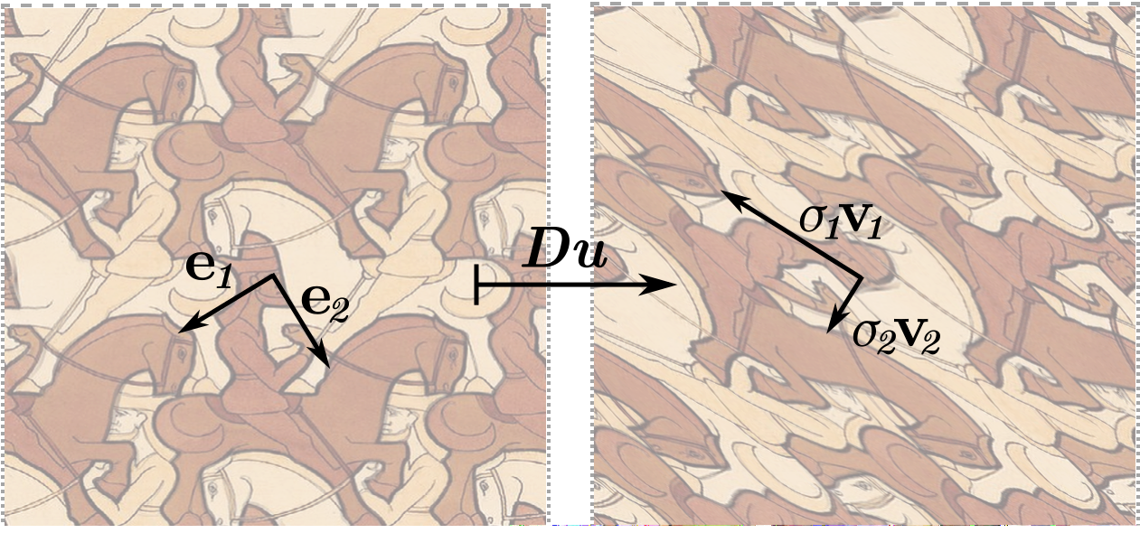 $Du(\v{e}_i) = \sigma_i \v v_i$ with $\sigma_i \ge 0;\;\v{e}_i, \v{v}_i$ orthonormal frames
$\{\sigma_1, \sigma_2\} = \{\min \beta, \max \beta\}$ where $\beta(v) =|Du(v)|/|v|.$
Maximum Principle for the Singular Values
- $Du$ is invertible iff both singular values are positive. Thus it suffices to preserve a positive lower bound on $\sigma_i$.
- The game plan: If $\sigma_1$ is the smaller singular value and attains a new minimum at $(x,t)$, then at this point we must have $\nabla^2 \sigma_1 \ge 0$, $\nabla \sigma_1 = 0$ and $\partial_t \sigma_1 \lt 0$. If we can show this contradicts the evolution equation for $\sigma_1$ then we're done.
Maximum Principle for the Singular Values
- The singular values provide a complete description of $Du$ up to isometry, so in order to be isometry-invariant, our coefficients must be of the form $a^{ij}(Du) = F(\sigma_1, \sigma_2)e_1^ie_1^j + F(\sigma_2, \sigma_1)e_2^ie_2^j.$
- Write $P = \partial_t - a^{ij}\nabla_i \nabla_j$. Differentiating $Pu=0$ and solving for $P\sigma_1$, we get $$P\sigma_1 = Q_F(\sigma)[\nabla^2u, \nabla^2u] + F \sigma_1 \left(\sigma_2^2 (\kappa \circ u) - \kappa\right)$$ for some quadratic form $Q_F(\sigma_1, \sigma_2)$.
- Since the curvature term does not depend on $\nabla^2u$, we need these two terms to be independently non-negative when $\nabla \sigma_1 = 0$.
MP for the Singular Values: Curvature Term
- Even if we assume constant curvature so $\kappa\circ u = \kappa$, the curvature term $F \kappa \sigma_1 (\sigma_2^2 - 1)$ has indefinite sign, so we're out of luck.
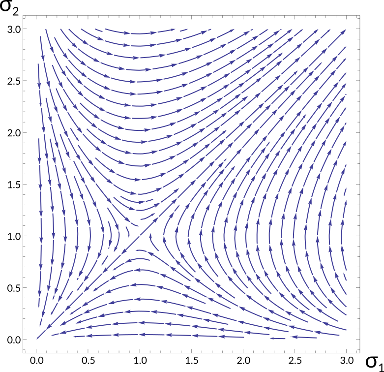 Considering the evolution of $(\sigma_1,\sigma_2)$ together and neglecting $\nabla^2u$, for $\kappa \gt 0$ the dynamics look like:
- Thus the eccentricity $\sigma_2/\sigma_1$ should behave nicely, but the determinant $\sigma_1 \sigma_2$ can diverge or degenerate.
- For $\kappa \lt 0$ we would have the opposite.
MP for the Singular Values: $\nabla^2u$ Term
- Now let's bring our attention to the quadratic term $Q_F(\sigma)[\nabla^2u,\nabla^2u]$. Assuming $\nabla \sigma_1 = 0$ and diagonalizing the quadratic form, we find $$ \begin{multline*} Q_{F}=\left[\frac{F\left(\sigma_1,\sigma_2\right)\sigma_1}{\sigma_2^{2}-\sigma_1^{2}}\right]y^{2} \\ +\left[\dot F^{1}\left(\sigma_2,\sigma_1\right)+\frac{2\left(\sigma_1+\sigma_2\right)}{\sigma_2^{2}-\sigma_1^{2}}F\left(\sigma_2,\sigma_1\right)\right]w^{2}\\ +\left[-\dot F^{1}\left(\sigma_2,\sigma_1\right)-\frac{2\left(\sigma_2-\sigma_1\right)}{\sigma_2^{2}-\sigma_1^{2}}F\left(\sigma_2,\sigma_1\right)\right]z^{2} \end{multline*} $$ for some components $w,y,z$ of $\nabla^2 u$.
MP for the Singular Values: $\nabla^2u$ Term
- Semi-positivity $Q_F \ge 0$ means each of these three coefficients must be non-negative; so (assuming $\kappa=0$) we find the required condition to preserve lower bounds:$$ \sigma_2\gt \sigma_1\implies-\frac{2}{\sigma_2-\sigma_1}\le\frac{\partial\log F\left(\sigma_2,\sigma_1\right)}{\partial \sigma_2}\le-\frac{2}{\sigma_2+\sigma_1}$$
- On the other hand, to preserve upper bounds we need: $$ \sigma_2\lt \sigma_1\implies-\frac{2}{\sigma_1+\sigma_2}\le\frac{\partial\log F\left(\sigma_2,\sigma_1\right)}{\partial \sigma_2}\le\frac{2}{\sigma_1-\sigma_2}$$
- Strictly speaking we haven't handled the case $\sigma_1 = \sigma_2$, where the SVD becomes irregular; but it turns out (by instead preserving bounds on $|Du(\cdot)|^2:UTM \to \mathbb R$ or similar) that there is no extra condition required.
Examples
Here are some functions $F$ defining flows that preserve diffeomorphisms in the flat setting:
- Our favourite is $F(\sigma_1,\sigma_2) = (\sigma_1 + \sigma_2)^{-2}$, which defines $\p_t u = (\sigma_1 + \sigma_2)^{-2} \Delta u$.
- Slightly simpler is $F(\sigma_1,\sigma_2) = (\sigma_1^2 + \sigma_2^2)^{-1}$, which defines $\partial_t u = |Du|^{-2} \Delta u$.
- Also interesting is $F(\sigma_1,\sigma_2) = 1/(\sigma_1(\sigma_1 + \sigma_2))$: in the case of area-preserving diffeomorphisms (i.e. $\sigma_1\sigma_2 = 1$) this flow coincides with mean curvature flow of $\mathrm{graph}(u) : M \to M \times M$, previously studied by Mu-Tao Wang [2001] for constant-curvature surfaces.
Existence & Regularity
- Well-known results for strongly parabolic systems provide short-time existence.
- To get long-time existence we need bounds on all derivatives.
- We just finished deriving bounds on the first derivatives using a maximum principle; but the nonlinearity makes extending this to higher derivatives impractical.
- Instead we will exploit the Schauder estimates with a bootstrap argument.
Hölder Spaces
- The Hölder ($C^{\alpha}$) norm is $$|u|_\alpha = \sup |u| + \sup_{X \ne Y} \frac{|u(X) - u(Y)|}{|X-Y|^\alpha}.$$
- If we use the parabolic distance function $$|(x,t) - (y,s)| = \max(|x-y|,\sqrt{|s-t|})$$then parabolic operators $P$ with $C^\alpha$ coefficients satisfy Schauder estimates $$|u|_{2,\alpha} := |u|_0 + |Du|_0 + |D^2u|_\alpha \lesssim |u|_0 + |Pu|_\alpha.$$
The Schauder Bootstrap
- Recall our quasilinear flow $Pu = \partial_t u - a^{ij}(Du) \nabla_i \nabla_j u = 0$
- Suppose we have shown that $|a^{ij}(Du)|_\alpha \lt \infty.$
- Then if $a$ is nice, Schauder $\implies |a^{ij}(Du)|_{1,\alpha} \lesssim |u|_{2,\alpha} \lt \infty.$
- Woohoo, a whole derivative for free! Now $Du$ satisfies an equation with $C^\alpha$ coefficients too, so $|a^{ij}(Du)|_{2,\alpha} \lesssim |u|_{3,\alpha} \lt \infty$.
- Repeating this, $u$ pulls itself up by its bootstraps, all the way to $C^\infty$.
- So we just need $Du \mapsto a(Du)$ to have bounded derivatives of all orders, and (the hard part) a Hölder bound on $X \mapsto a(Du(X))$.
Hölder Estimate: The archetype
A useful stepping stone to a $C^\alpha$ estimate is a weak Harnack inequality:

Hölder Estimate: The archetype
Theorem: If $Pu = f$ then $|u|_\alpha \lesssim |u|_0 + |f|_0.$
Proof. Note that $\sup_{Q(4R)}u - u,$ $u - \inf_{Q(4R)} u$ are positive solutions of $Pu = \pm f$ on $Q(4R)$. Then weak Harnack gives
$$\begin{align} \fint{\Theta\left(R\right)}\left(\sup_{Q(4R)}u-u\right) & \le C\left(\sup_{Q(4R)}u-\sup_{Q(R)}u+|f|_0 R^2\right) \tag{1}\\ \fint{\Theta\left(R\right)}\left(u-\inf_{Q(4R)}u\right) & \le C\left(\inf_{Q(R)}u-\inf_{Q(4R)}u+|f|_0 R^2\right)\tag{2} \end{align}$$
$$\begin{align} \osc_{Q\left(4R\right)}u & \le C\left(\osc_{Q\left(4R\right)}u-\osc_{Q\left(R\right)}u+2|f|_0 R^2 \right) \tag{1+2} \\ \osc_{Q(R)} u & \le (1-C^{-1}) \osc_{Q(4R)} u + 2|f|_0 R^2. \end{align}$$
Iterating this gives $\osc_{Q(R)} u \le C(\osc_{Q(R_0)} u,|f|_0) \left(\frac{R}{R_0}\right)^{\alpha}.$
Hölder estimate for the coefficient
- For now on, fix $M= \mathbb T^2$ and $a^{ij} = r^{-2}g^{ij}$ where $r = \sigma_1 + \sigma_2$. Assuming bounds $0 \lt \lambda \le r \le \Lambda$, a Hölder estimate for $r$ will get the bootstrap started.
- Evolution equation for $r$ can be written $$Pr = -\frac{2}{r^3}\left(|\nabla r|^2 + r \nabla r \times \nabla\theta\right) - \frac 1 r |\nabla \theta|^2 \tag{*}$$ where $\theta$ is the rotation angle between the singular frames of $Du$.
- Thanks to our choice of $a^{ij}$, $P \theta = 0$!
- Thus we get an estimate for $|\theta|_\alpha$; but this doesn't tell us anything about the size of $\nabla \theta$, so we can't just treat (*) as a linear equation.
- We need to be a little cleverer.
Hölder estimate for the coefficient
- Recall that the Hölder estimate via weak Harnack uses sub- and supersolutions separately.
- We can see from (*) that $r$ is a subsolution but not a supersolution.
- By considering $r^p$ for $p \in (0,1)$ we can add $|\nabla r|^2$ terms to the evolution equation. By also switching to the divergence-form operator $L = \partial_t - \nabla_i (a^{ij} \nabla_j \cdot)$ we can add enough to overpower the $-2r^{-3}|\nabla r|^2$.
- By subtracting a multiple of $\theta^2$ we can add $|\nabla \theta|^2$ terms.
- Restricting to small enough radii, we can find $c \gt 0, p\gt 0$ such that $w=r^p - c\theta^2$ satisfies $Lw \ge 0$, and $Lr^2 \le 0$.
Hölder estimate for the coefficient
- The weak Harnack inequality gives $$\begin{align} \fint{\Theta\left(R\right)}\left(w-\inf_{Q\left(4R\right)}w\right)&\le C\left(\inf_{Q\left(R\right)}w-\inf_{Q\left(4R\right)}w\right)\\ \fint{\Theta\left(R\right)}\left(-r^{2}+\sup_{Q\left(4R\right)}r^{2}\right)&\le C\left(-\sup_{Q\left(R\right)}r^{2}+\sup_{Q\left(4R\right)}r^{2}\right). \end{align}$$
- Since $r \mapsto r^p$ is bi-Lipschitz on $[\lambda,\Lambda]$, by increasing $C$ we can get $$ \begin{align*} \fint{\Theta\left(R\right)}\left(r-\inf_{Q\left(4R\right)}r\right) & \le C \left(\inf_{Q\left(R\right)}r-\inf_{Q\left(4R\right)}r+\sup_{Q\left(4R\right)}\theta^{2}\right)\\ \fint{\Theta\left(R\right)}\left(-r+\sup_{Q\left(4R\right)}r\right) & \le C\left(\sup_{Q\left(4R\right)}r-\sup_{Q\left(R\right)}r\right). \end{align*} $$
- Now add!
Hölder estimate for the coefficient
- Adding yields $$\osc_{Q\left(4R\right)}r\le C'\left(\osc_{Q\left(4R\right)}r-\osc_{Q\left(R\right)}r+\sup_{Q\left(4R\right)}\theta^{2}\right)$$ for all $R \le R_0$, so rearranging and iterating as before using $\sup_{Q(R)} \theta^2 \le C(|\theta|_\alpha) R^\alpha$ we get $$\osc_{Q(R)} r \le C(|\theta|_\alpha, \lambda, \Lambda) R^\alpha.$$
- So we have a uniform Hölder estimate for the coefficients, and the bootstrap goes through.
Long-time behaviour
- When $F$ is symmetric (so that $\partial_t u = F(\sigma_1,\sigma_2)\Delta u$), the energy $E=\int |Du|^2$ satisfies $E'(t) = - \int F |\Delta u|^2,$ so we get smooth convergence to a harmonic limit on some sequence of times.
- On a flat surface, much integration by parts (along with the Ladyzhenskaya inequality) yields $$\frac{d}{dt}\int |D^2 u|^2 \le -C_1 \left(1- C_2 \int |D^2 u|^2\right)\int |D^3 u|^2.$$
- Thus for initial data with $D^2 u$ small enough in $L^2$, the quantity $\int |D^2 u|^2 = \int |F^{-1} \p_t u|^2 $ converges exponentially to zero.
Long-time behaviour
The exponential convergence $\|\p_t u\|_{L^2} \to 0$ along with our bounds $|D^k u|_0 \le C_k(u(0))$ is now enough to get smooth convergence:
- By the interpolation inequality $|\p_t u|_0^2 \le |D\p_t u|_0 \|\p_t u\|_{L^2}$ we conclude $|\p_t u|_0 \to 0$ exponentially and thus $|u(t)-u_\infty|_0 \to 0$ exponentially.
- Interpolating $$|D^k(u(t) - u_\infty)|_0 \lesssim C_{2k} |u(t) - u_\infty|_0$$ we find that all derivatives converge exponentially.
Using the $C^\infty$ estimates, we can show that the solution operator $(u_0, t) \mapsto u(t)$ is continuous in the $C^\infty$ topology; so the flow is a deformation retract of $\mathrm{Diff}^+(\mathbb T^2)$ on to $SL(2,\mathbb Z) \times \mathbb T^2$.
Thanks for listening!
Further information
- Fiddle with donuts at a.carapetis.com/diff_flow/
- Read some of the details at arxiv.org/abs/1609.08317
- (thesis coming soon!)
Reference
[2001] Mu-Tao Wang. Deforming area preserving diffeomorphism of surfaces by mean curvature flow